Medallion Architecture in Microsoft Fabric: From Ingestion to Secured Reporting

A practical, end-to-end walkthrough of building the bronze, silver, and gold layers in Microsoft Fabric, including data masking and row-level security in the gold layer.

Picture of Sabhye Singhal<br>Lead Data Engineer, Expert-Extend

Sabhye Singhal
Lead Data Engineer, Expert-Extend

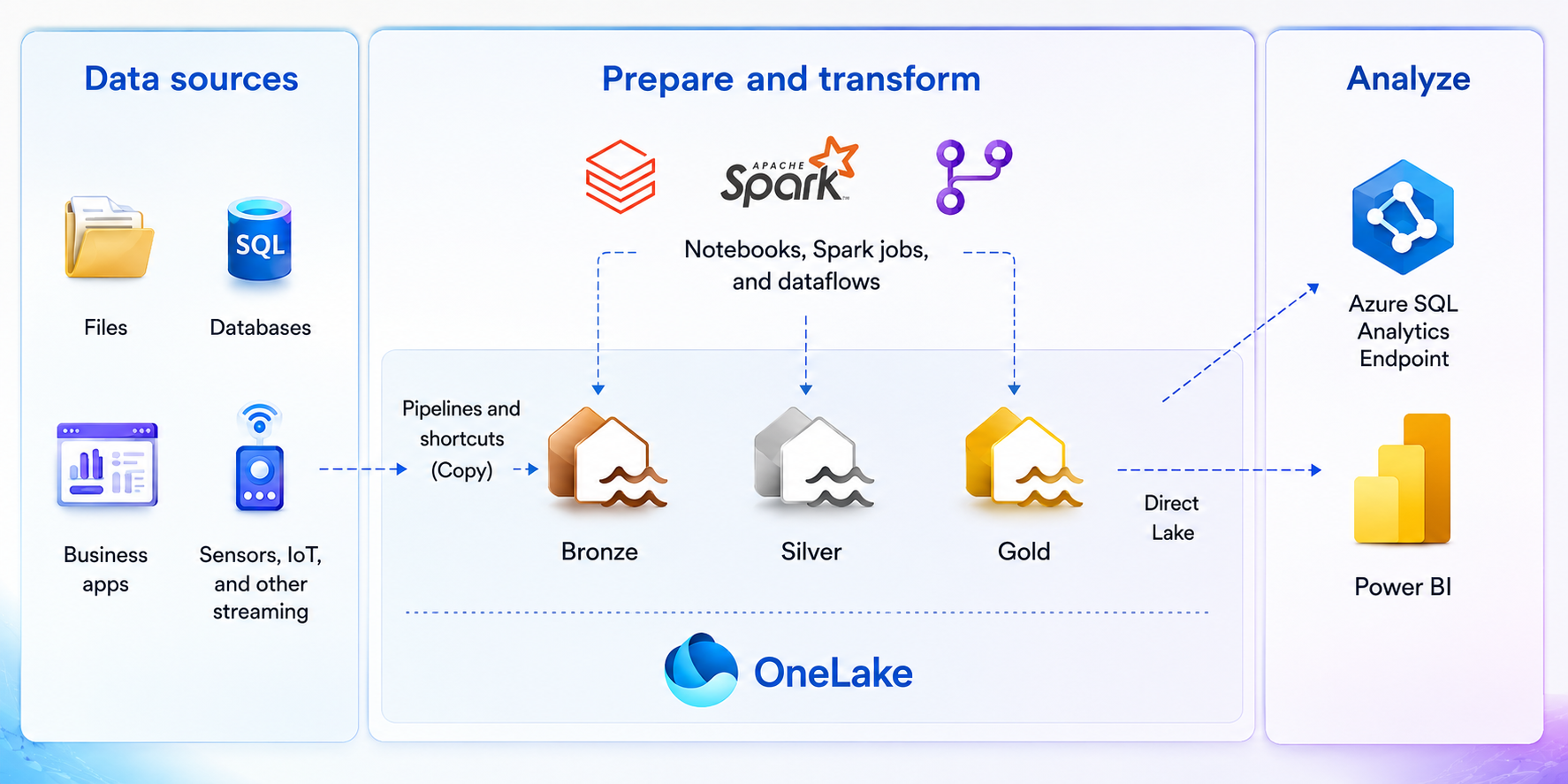
Medallion architecture diagram in Microsoft Fabric: data sources flow via pipelines and shortcuts into Bronze, Silver and Gold layers in OneLake, then to Power BI and the SQL analytics endpoint.

Table of Contents

What Is Medallion Architecture?

The goal of medallion architecture is to incrementally improve the structure and quality of data. Think of medallion architecture as a three-stage cleaning and organizing process for your data. Each layer makes your data more reliable and easier to use.

1. Bronze (Raw): Store everything exactly as it arrives. No changes are allowed. 

2. Silver (Enriched): Fix errors, standardize formats, and remove duplicates.

3. Gold (Curated): Organize for reports and dashboards. 

This architecture involves Extract, Transform, and Load of the source data. The source data can be both internal (One Lake or on-prem database) or external (Azure Data Lake Store Gen2, Amazon S3, Google Cloud Storage, Azure SQL database) storage systems. 

How Data Flows Through the Layers

Extract: Source to Bronze

Extract data from the source side to the bronze layer Lakehouse using shortcuts or through pipelines using copy data activity and save it in delta format 

In the bronze layer, you store data in its original format, which might be either tables or files. Tables will be used to store structured datasets (CSV, Parquet, or Delta), and files will be used to store semi-structured or unstructured datasets (JSONs, logs, PDFs, images, IOT readings). 

In the bronze layer, you can have smaller files because of the raw nature of the data, as long you focus data modification and preparation with Spark. 

Transform: Bronze to Silver

Transform the data from Bronze lakehouse to Silver lakehouse, either using a notebook or Dataflow Gen2.  

In Silver layer, you store the data as delta tables after applying transformation rules such as data quality checks, null checks, removing duplicate records, appropriate aggregations as per the business requirements, etc. 

Delta tables use V-Order write-time optimization to the Parquet file format. That optimization enables fast reads by Fabric compute engines, such as Power BI, SQL, Apache Spark, and others. 

Load: Silver to Gold

Once the data is transformed, we will load the data into the gold layer. 

– This layer will be a warehouse, unlike bronze and silver layers, which were lakehouses.

Data gets loaded to the gold layer by either using a pipeline or through dataflow Gen2. 

– The gold layer will be the SQL analytics endpoint for the semantic models or the reports in our workspace.

– The gold layer will contain the Star schema fact and dimension tables and any relationships in between them.

Purpose of the blog

Technical guide on how to implement Medallion architecture in Microsoft Fabric.  

Technical guide on how to implement data masking and row-level security in the gold layer. 

Identification of the limitations in the previous architecture and the advantages of the current architecture.

Implementing Medallion Architecture in Microsoft Fabric, Step by Step

Building the Bronze Layer (Raw Data)

– This layer contains a raw data or a copy of the data from the source side without any kind of transformations applied. 

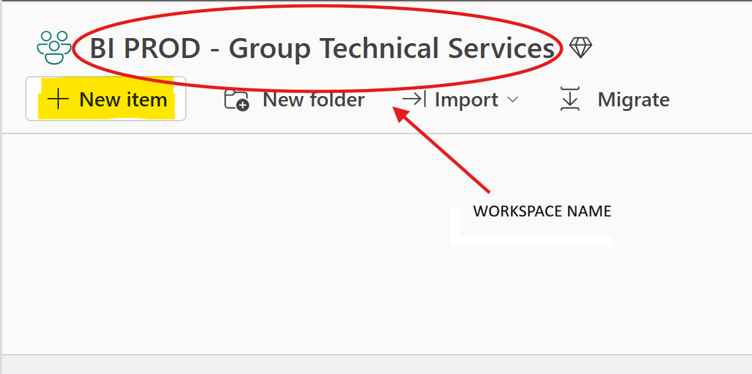
– Assuming we have already created a workspace, click on new item as shown below.

Microsoft Fabric workspace with the New item button selected to create a lakehouse.

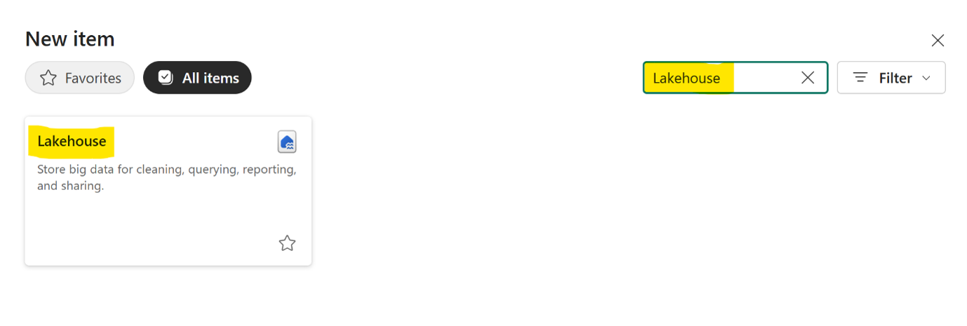
Search for Lakehouse item and click on that item.

Fabric New item panel with Lakehouse selected from the item type list.

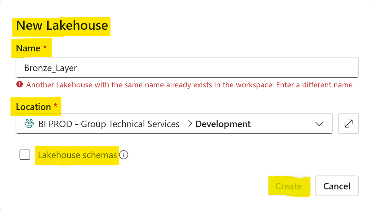
Give the name as Bronze Layer, provide the location where you want to save the item in the workspace, check/uncheck Lakehouse Schemas (Schemas let you manage and reference objects in your lakehouse more easily. You can use a default schema to automatically fill in file paths when referencing a data object in code) depending upon the use case and click on Create. You will see a new item of Lakehouse being created.

Create lakehouse dialog with the name set to Bronze Layer and the Lakehouse schemas option shown.

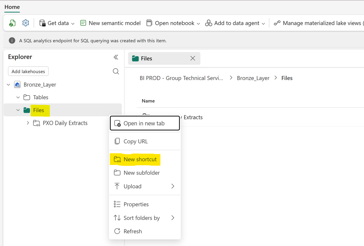
Go inside that item and click on the three dots beside the Files Folder. Click on New Shortcut.

New shortcut data source screen with a SharePoint folder selected as the source.
Bronze Layer lakehouse Files folder with the three-dot menu open on the New shortcut option.

Go inside that item and click on the three dots beside the Files Folder. Click on New Shortcut.

New shortcut data source screen with a SharePoint folder selected as the source.

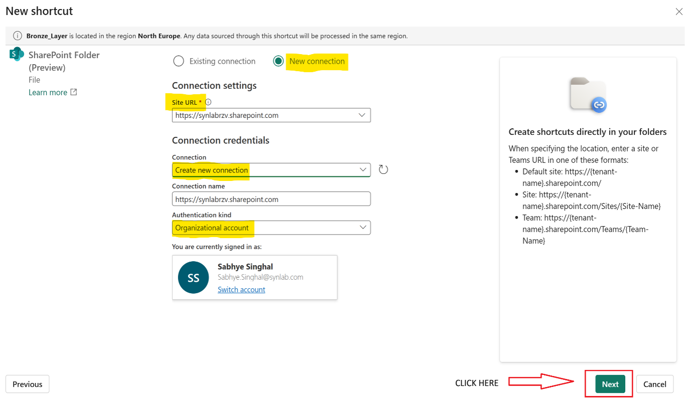
Since initially we won’t have an existing connection, we will create a new connection and provide the authentication kind as Organizational account. Click on the Next button.

Shortcut connection setup with authentication kind set to Organizational account.

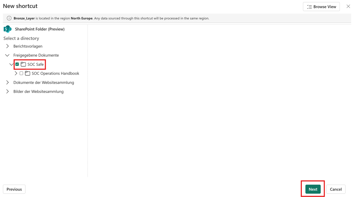
Select an appropriate directory of which you want to create a shortcut. Click on Next button. 

Shortcut wizard step for selecting the source directory to shortcut into the lakehouse.

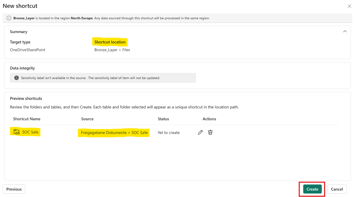
It will summarize with the location of the shortcut. Click on Create button.

Shortcut summary screen showing the target location before creating the shortcut.

– A new shortcut will be created with the same name as the directory name at the source side. In our case, we have already made a shortcut with a different directory as the source, hence it won’t be seen in the image below. 

Bronze Layer lakehouse Files folder showing the newly created shortcut to the source directory.

Similarly, we can do for other data sources as well.

Building the Silver Layer (Transformed Data)

– This layer contains transformed data. This means it will have the data after implementing all kinds of transformations, such as data quality checks, aggregations, joins, unions, data type checks, null checks, etc. 

To transform the data, we can either use a Spark Notebook or a Dataflow Gen2. In our case, we are creating a PySpark Notebook.

To create this layer, again click on new item as shown above in Bronze Layer. 

– Search for the Lakehouse item and click on that item. 

– Give the name as Silver Layer, provide the location where you want to save the item in the workspace, check/uncheck Lakehouse Schemas as per the use case, and click on Create. You will see a new item of Lakehouse being created. 

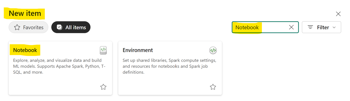
– Now, again click on the new item as shown above in the Bronze Layer. 

Fabric New item search showing the Notebook option for the Silver layer

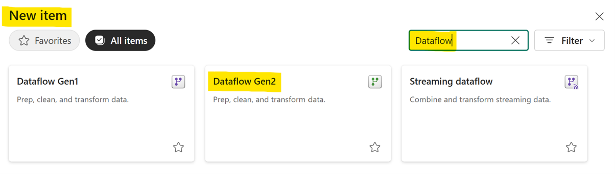
Search for Notebook/Dataflow Gen2.

Fabric New item search showing the Dataflow Gen2 option for the Silver layer transformation.

For Notebook:

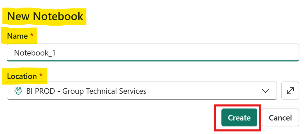
– Enter the name of the item and the location where you want to save.

New notebook dialog with fields for the notebook name and save location.
Fabric New item search showing the Dataflow Gen2 option for the Silver layer transformation.

Click on Create button.

For Dataflow Gen2:

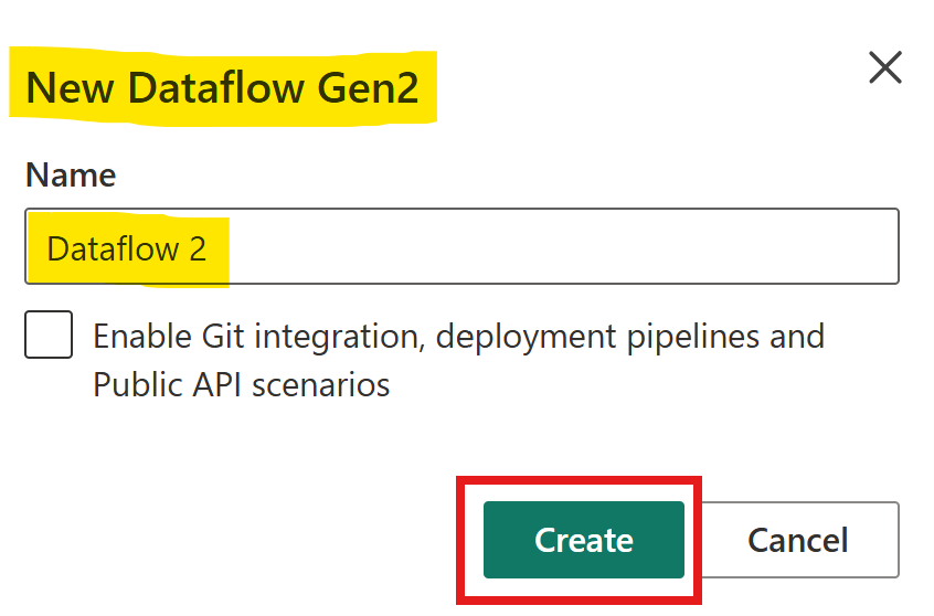
Enter the name of the dataflow and uncheck Git integration box.

New Dataflow Gen2 dialog with the Git integration checkbox unchecked.

Click on Create button.

– You will see a new item of Notebook/Dataflow Gen2 being created.

– Open the item

For Notebook:

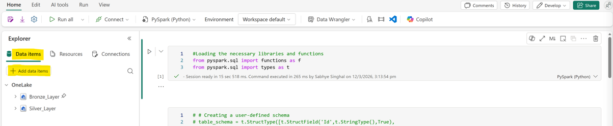
– Click on Data items

Fabric notebook editor with the Data items button selected to attach lakehouses.

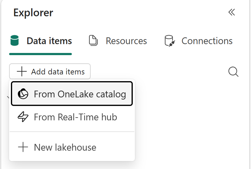
Click on the OneLake Catalog

OneLake catalog dialog for selecting lakehouses to load into the notebook.

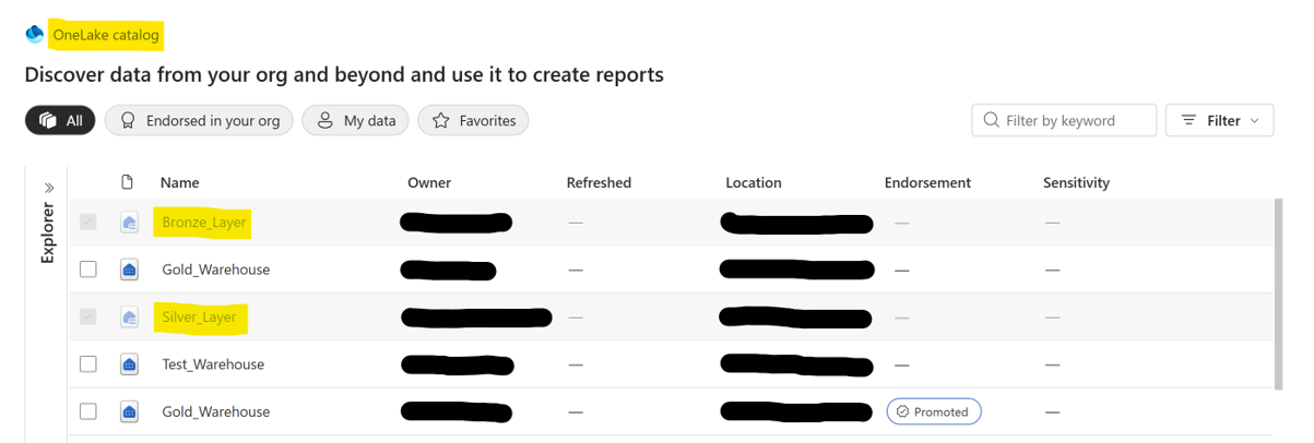
Choose the Bronze and Silver Layer lakehouse as the data items to load to the Notebook. Click on the Add button.

OneLake catalog with the Bronze Layer and Silver Layer lakehouses selected to add to the notebook.

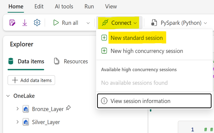
You will see the data items as shown below added. Then, click on connect tab and on New Standard Session to connect to processing engine where the script will run.

Notebook with Bronze and Silver lakehouses attached and the New standard session connect option.

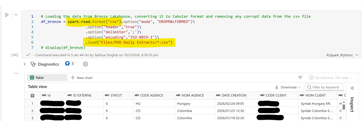
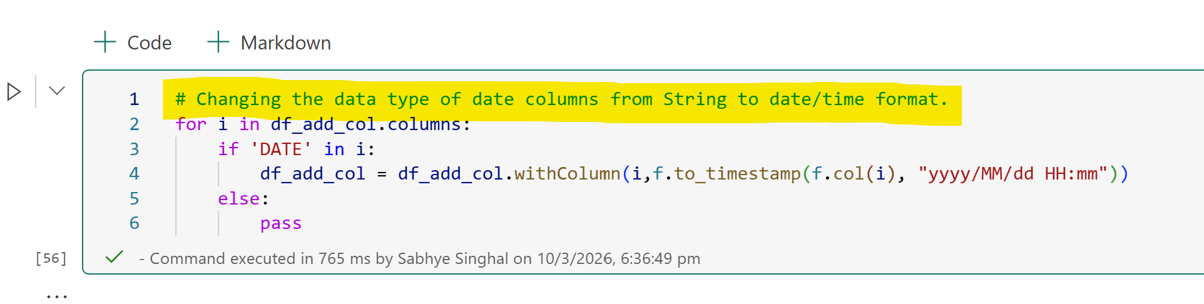
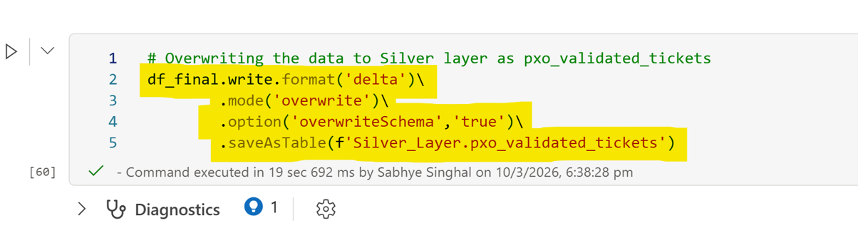
Write the commands of loading the data from bronze layer, transforming the data on top of the loaded dataframe and  writing the dataframe to Silver Layer in the notebook cells as shown.

PySpark notebook cell reading CSV data from the Bronze lakehouse into a dataframe, with a table preview (sensitive fields redacted).
PySpark notebook cell looping through columns to convert date fields from string to timestamp format.
PySpark notebook cell writing the transformed dataframe to the Silver layer as a Delta table in overwrite mode.

For Dataflow Gen2:

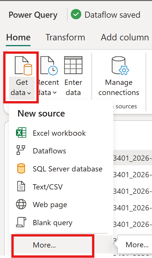
Click on Get data. Click on More. 

Dataflow Gen2 Get data screen with the More option selected.

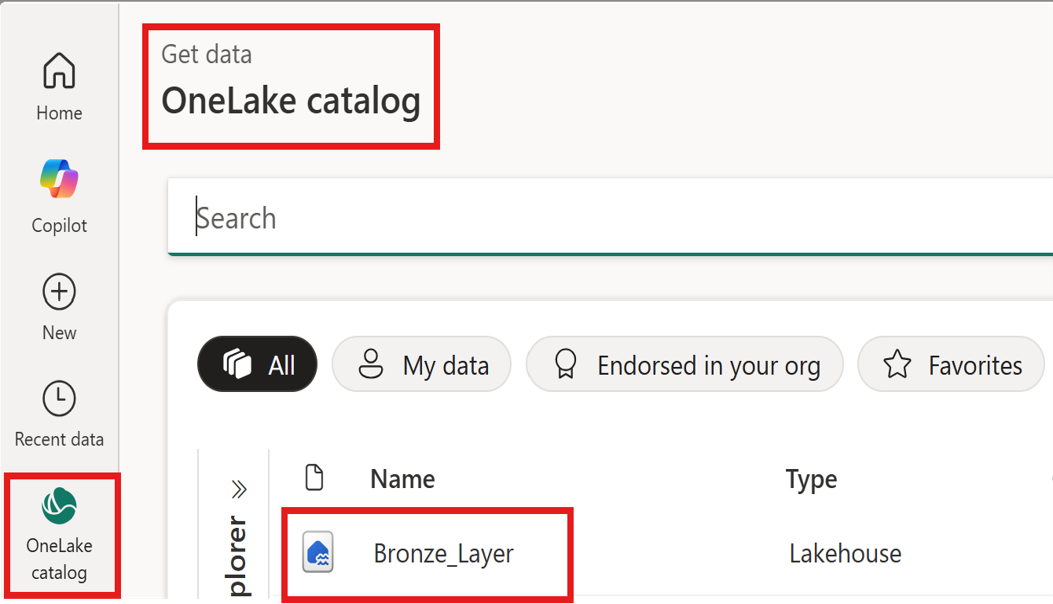
Click on OneLake catalog. Choose Bronze layer lakehouse item.

Dataflow Gen2 OneLake catalog with the Bronze Layer lakehouse selected as source.

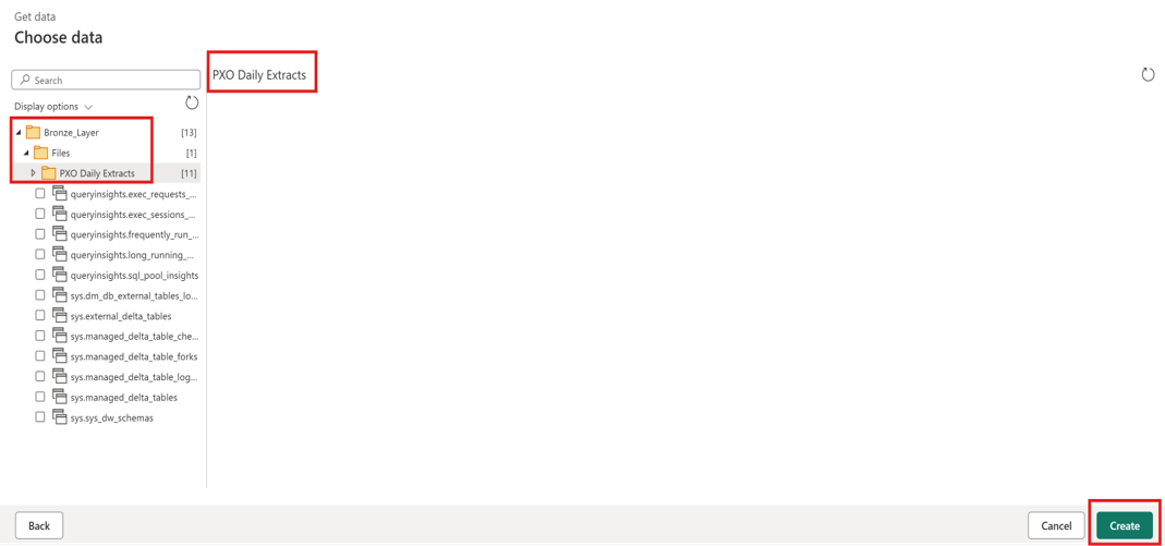
Choose appropriate directory/files.Click on Create button.

Dataflow Gen2 source selection of the directory and files from the Bronze layer.

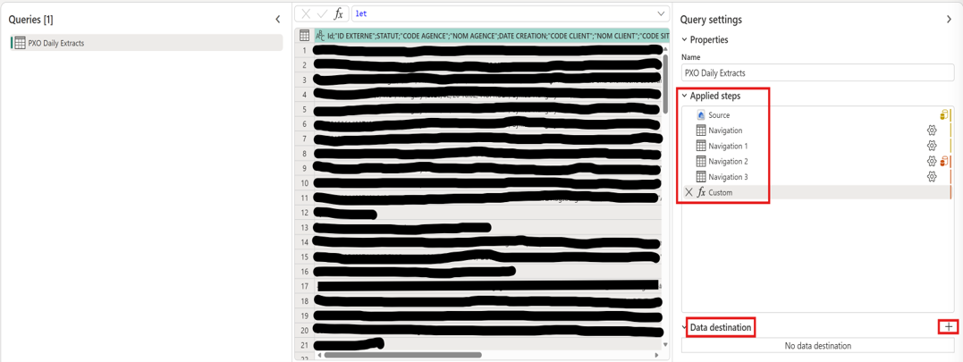
Write commands to do transformations as per business use case and click on ‘+’ sign besides data destination.

Dataflow Gen2 editor showing transformation steps and the add data destination button.

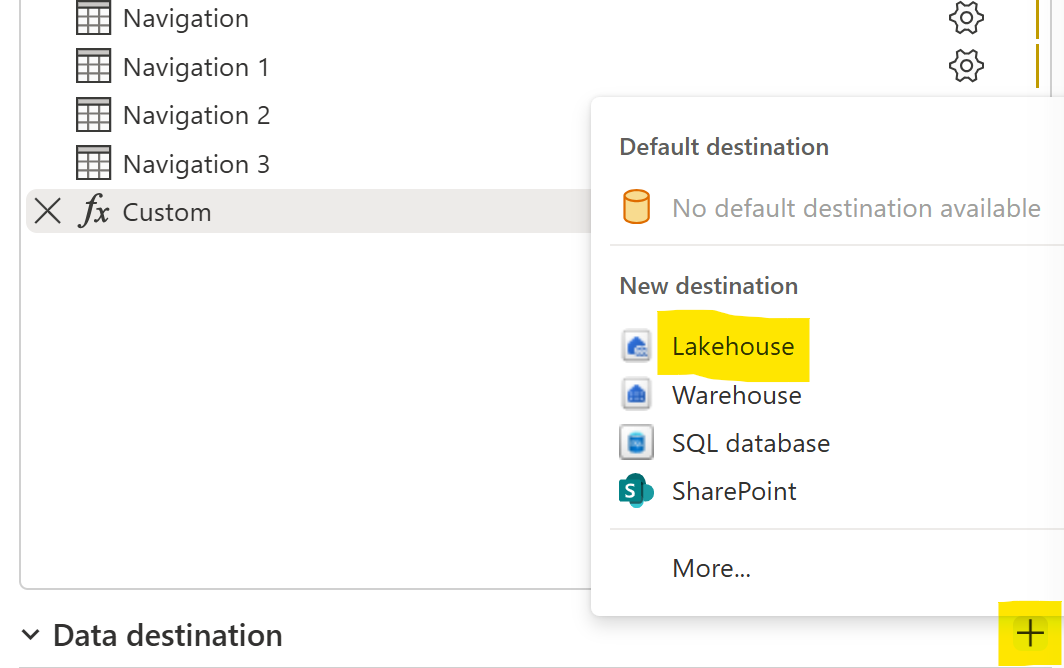
Click on more and choose Lakehouse.

Dataflow Gen2 data destination options with Lakehouse selected.

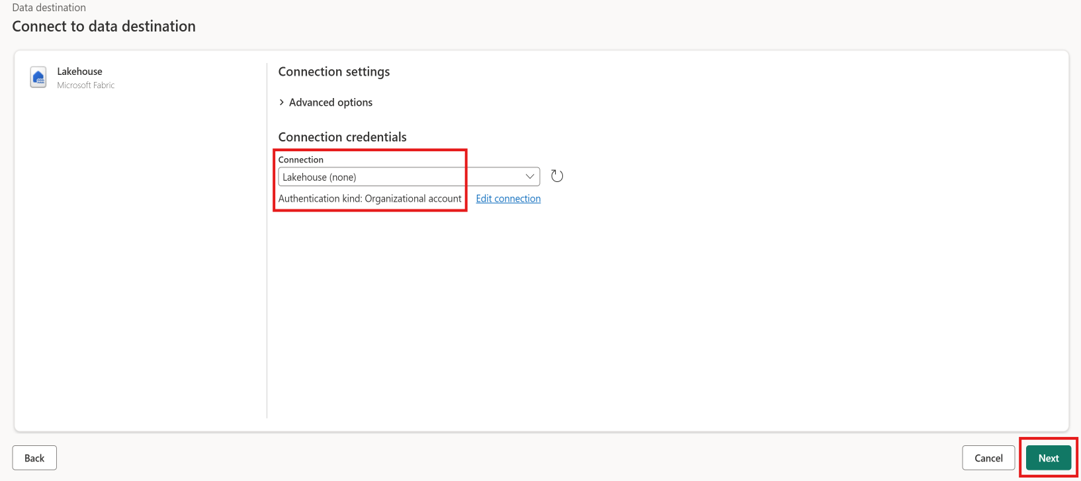
Click on the Next button and choose existing lakehouse connection credentials.

Dataflow Gen2 destination connection setup using existing lakehouse credentials.

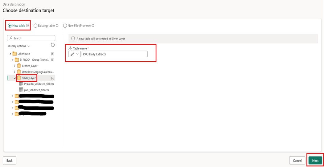
Go to the appropriate workspace and lakehouse location and choose Silver Layer as the destination. 

– You can choose between a new table, an existing table, or a new file. In our case, we will be choosing a new table.  

– Click on Next button.

Dataflow Gen2 destination set to the Silver Layer lakehouse with the New table option.

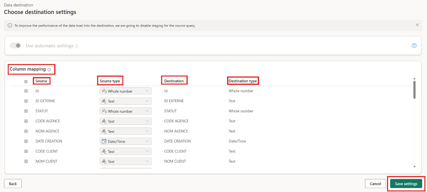
It will map the columns with appropriate column data types. You can change the data types according to the use case. Click on save settings.

Dataflow Gen2 column-to-data-type mapping screen for the destination table.

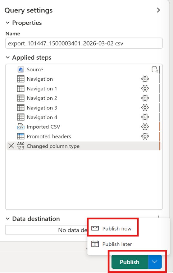
– Click the publish button

Dataflow Gen2 editor with the Publish button.

We will schedule and run the Notebook/Dataflow Gen2 using data pipelines. It is mentioned in detail under gold layer.

Building the Gold Layer (Curated Warehouse)

– This will be a warehouse. It will only contain the data that is for immediate use in the semantic model and reports. It will contain the data that is necessary for analysis purposes. 

– This will get updated either daily, weekly, or monthly, depending on the use case. 

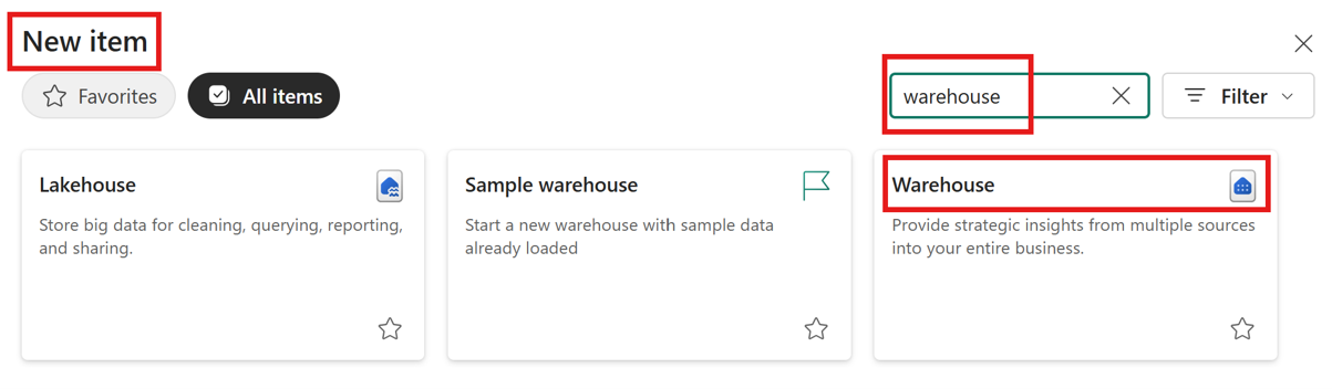
– To create this layer, again click on new item as shown above in Bronze Layer. Search for a warehouse.

Fabric New item search showing the Warehouse option for the Gold layer.

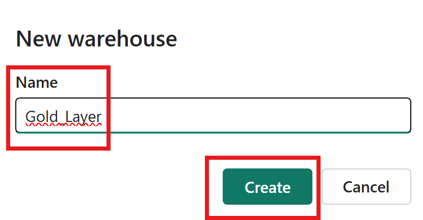
– Name the warehouse and click on the Create button. 

Create warehouse dialog with the name field and Create button.

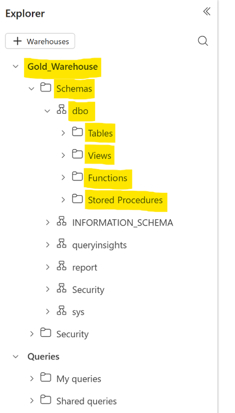
It will contain dbo as the default schema. Under this schema, we can create tables, views, functions, or stored procedures. 

New Fabric warehouse showing the default dbo schema for tables, views, functions and stored procedures.

Since we are not doing any type of transformations on top of data stored in the Silver layer, we will directly migrate the data from the Silver layer to the Gold layer using a copy data activity in data pipelines. 

– In case one wants to do some kind of column selection or renaming or create additional columns on top of existing ones, they can do it using a Notebook/dataflows before moving the data to the Gold layer. Steps will remain the same as mentioned under the Silver layer. 

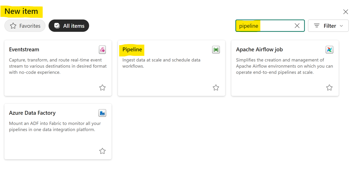
– Now, again click on the new item as shown above in Bronze Layer. Search for pipeline. 

Fabric New item search showing the Data pipeline option.

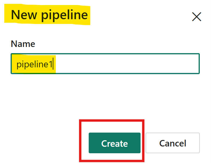
– Name the pipeline and click on the Create button.

Create data pipeline dialog with the name field and Create button.

We will be creating two pipelines here. One to schedule the notebook/dataflow and another to copy the data from the Silver layer to the Gold Layer. 

Empty Fabric data pipeline canvas ready for adding activities.

Bronze to silver layer pipeline

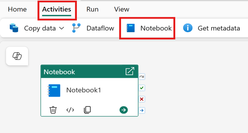
– Go to the activities tab. Click on Notebook. 

Bronze-to-Silver pipeline with the Notebook activity added on the activities tab.

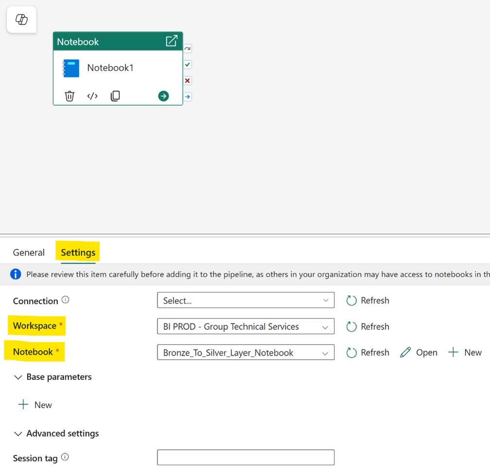
Go to the Settings tab. 

– Choose the workspace where your notebook/dataflow resides. 

– Choose the notebook/dataflow that you want to schedule for run. 

Notebook activity Settings tab with the workspace and notebook to schedule selected.

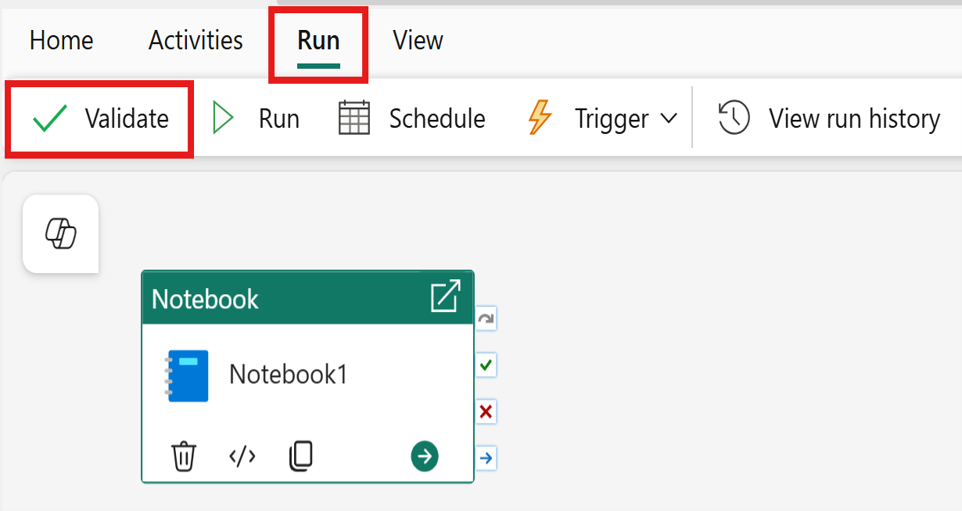
– Go to the Run tab. Click on ” Validate “ to check for any errors in your pipeline activities. 

Pipeline Run tab with the Validate button to check activities for errors.
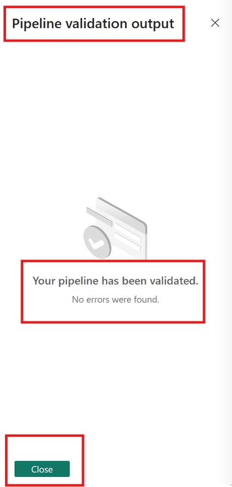
Pipeline validation output confirming no errors in the activities.
Pipeline Run tab with the Validate button to check activities for errors.

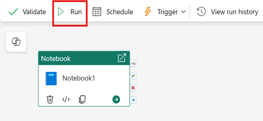
If no errors, click on run.

Pipeline Run tab with the Run button.
Pipeline Run tab with the Validate button to check activities for errors.

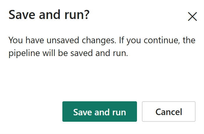
This will ask you to save and run your notebook/dataflow for the first time. Click on save and run. 

Save and run confirmation prompt for the notebook pipeline.

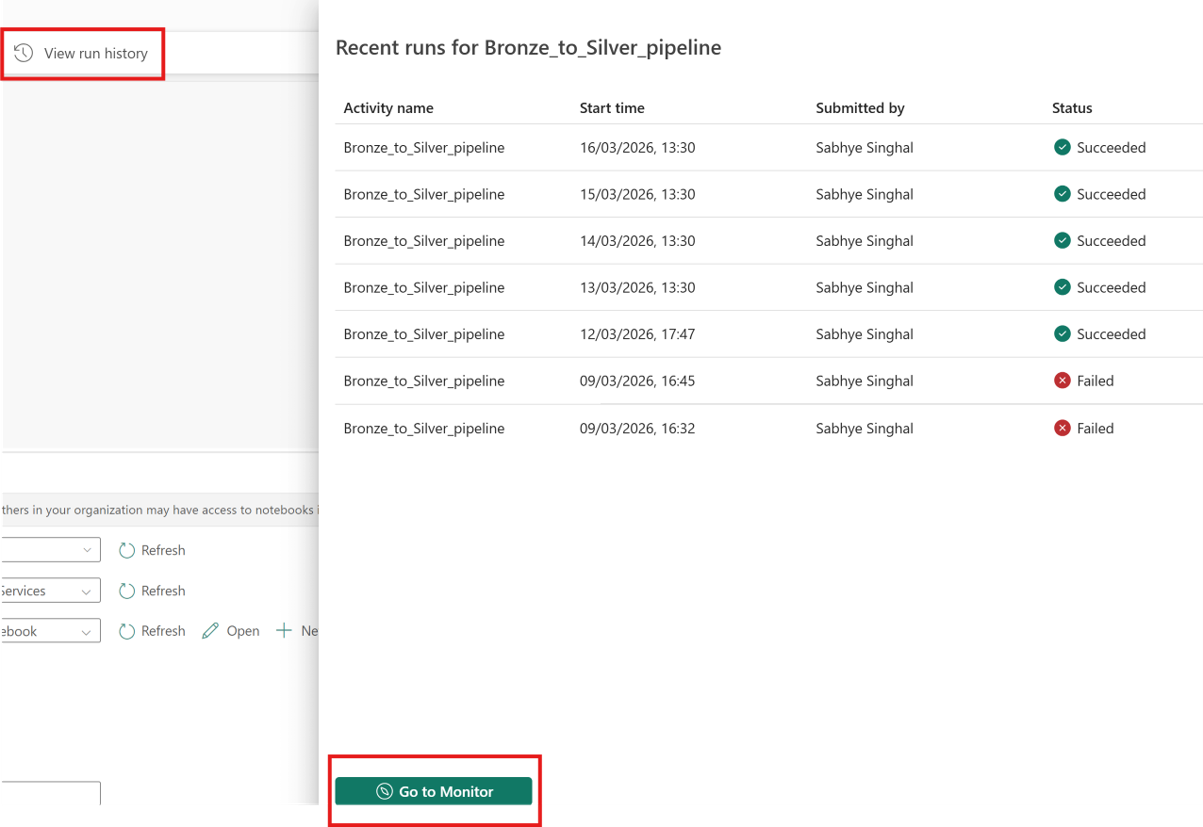
You can monitor the runs by going to View run history and then clicking Go to Monitor.

Pipeline run history and Monitor view showing the run status.

Silver to Gold Layer pipeline

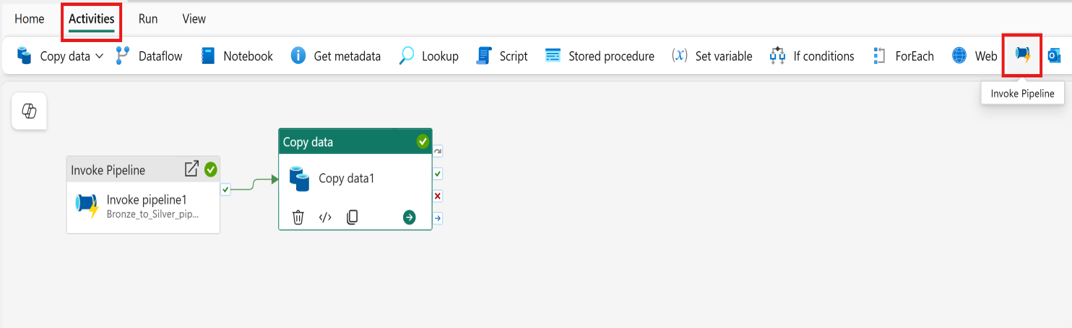
Go to activities tab. Click on Invoke pipeline. 

Silver-to-Gold pipeline with the Invoke pipeline activity added on the activities tab.

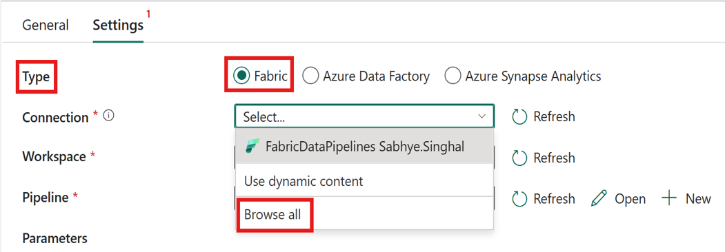
Click on Settings. Type will be fabric.  

For Connection, click on Browse all.

Invoke pipeline Settings with type set to Fabric and the Browse all connection option.

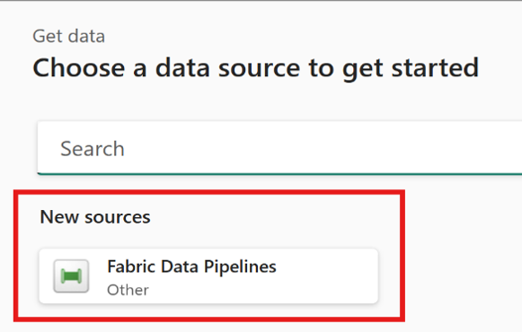
Click on Fabric data pipeline. 

Connection picker with Fabric data pipeline selected.

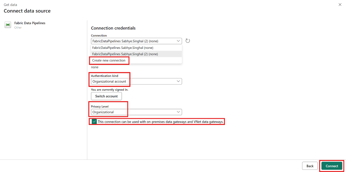
Create a new connection. Click on Connect.

New connection dialog for the Fabric data pipeline with the Connect button.

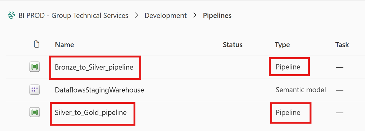
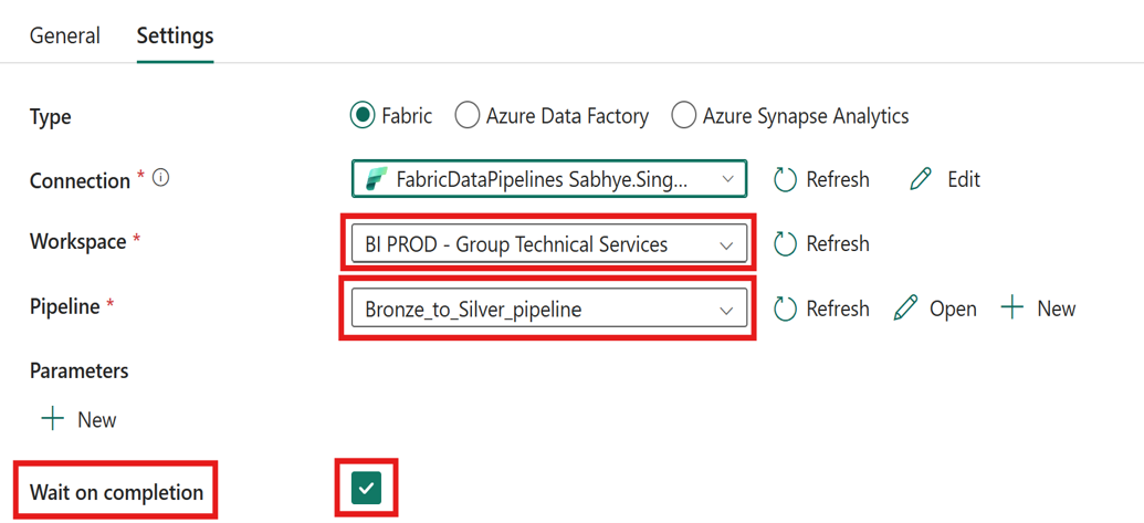
Choose the appropriate workspace. Choose bronze_to_silver layer pipeline. Check mark wait on completion. This will invoke bronze to silver layer pipeline.

Invoke pipeline settings with the bronze_to_silver pipeline selected and Wait on completion checked.

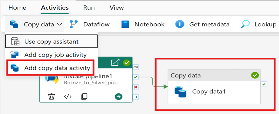
Now, Click on copy data. Click on Add copy data activity.

Pipeline canvas with the Copy data activity being added.

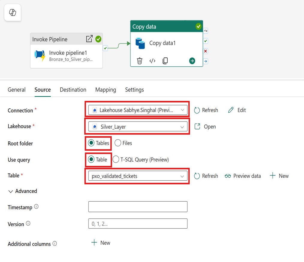
Click on Source.

Connection will be Lakehouse and Lakehouse will be Silver Layer Lakehouse. 

We are saving our data as tables in silver layer. So, our root folder will be Tables, and the query will be Table.

We will choose our praxedo table from the dropdown. 

Copy data Source settings with the Silver Layer lakehouse and the source table selected from Tables.
Pipeline canvas with the Copy data activity being added.

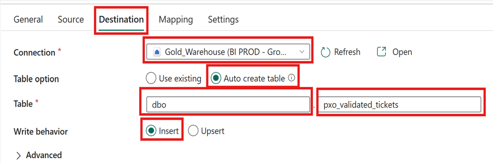
Now, choose destination.

Connection will be Gold layer. Table option will be Auto create table.

Provide the schema name and the table name. Write behaviour will be insert.

Copy data Destination settings with the Gold warehouse, Auto create table option and Insert write behaviour.

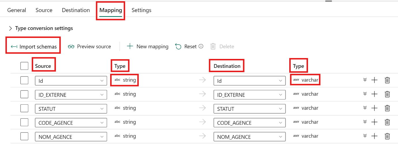
Click on Mapping. Click on import schemas. This will map the source and destination table columns automatically.

Copy data Mapping tab after importing schemas to map source and destination columns.

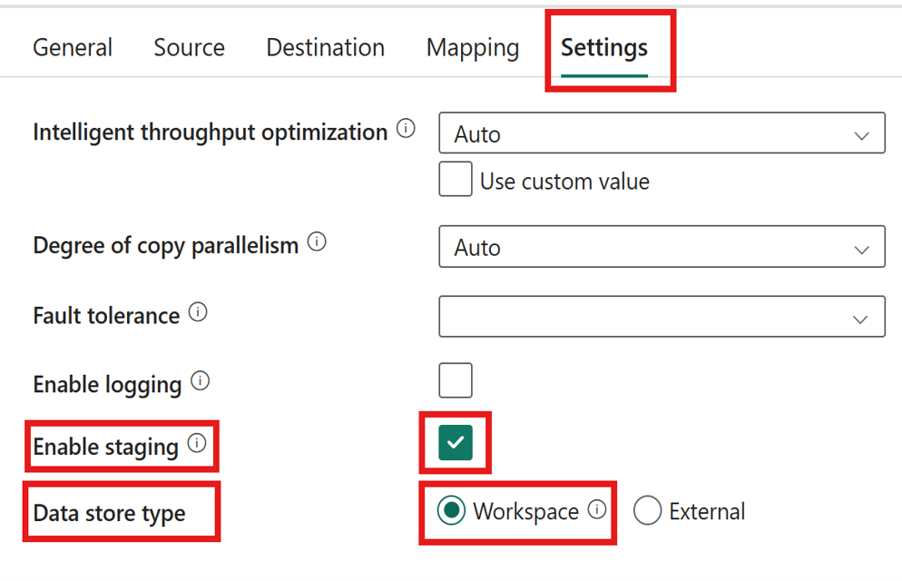
Ensure that under Settings tab, Enable staging is ON and data store type is Workspace.

Copy data Settings tab with Enable staging on and data store type set to Workspace.

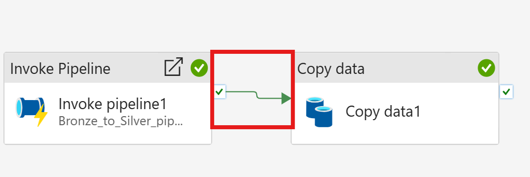
Now create an arrow from Invoke pipeline to copy data activity. These activities will then run in sequence.

Pipeline canvas with an arrow connecting the Invoke pipeline activity to the Copy data activity in sequence.

Go to Run tab. Click on validate to check for any errors in your pipeline activities as shown in previous steps.

If no errors, click on run. This will ask you to save and run your pipeline for the first time. Click on save and run. Bronze to Silver layer pipeline will also run and that will simply overwrite the data from Bronze to Silver layer. 

Once the run is successful, go back to Activities tab and click on copy data activity.

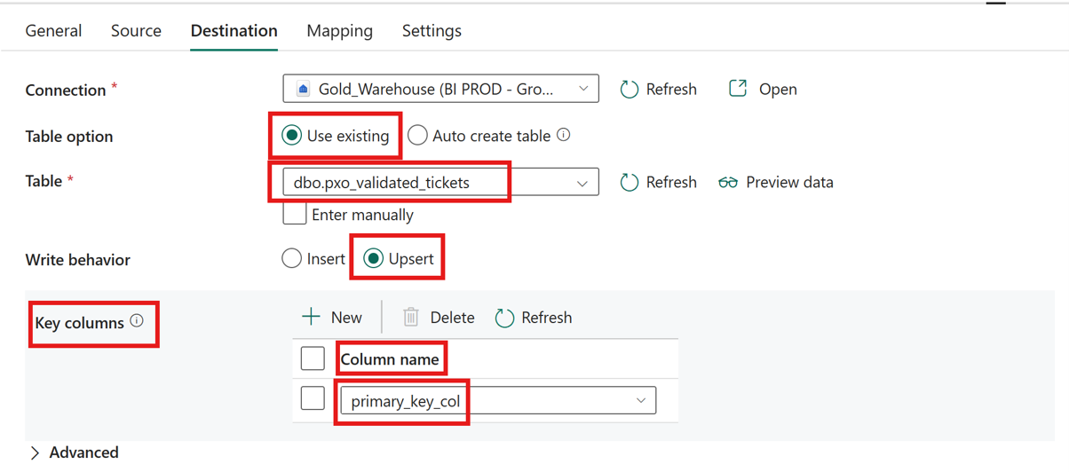
Now, change the table option from Auto create table to Use existing and choose the appropriate destination table from the drop down. 

Also, change the write behaviour from insert to upsert. It will ask for Key columns which will help it to analyze which data is to insert and which data to update accordingly.

Copy data Destination updated to Use existing table with Upsert write behaviour and key columns selected.

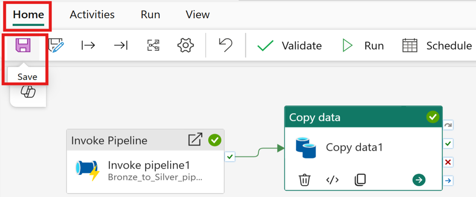
Go back to Home tab.

Click on Save button.

This will save your pipeline.

Pipeline Home tab with the Save button.

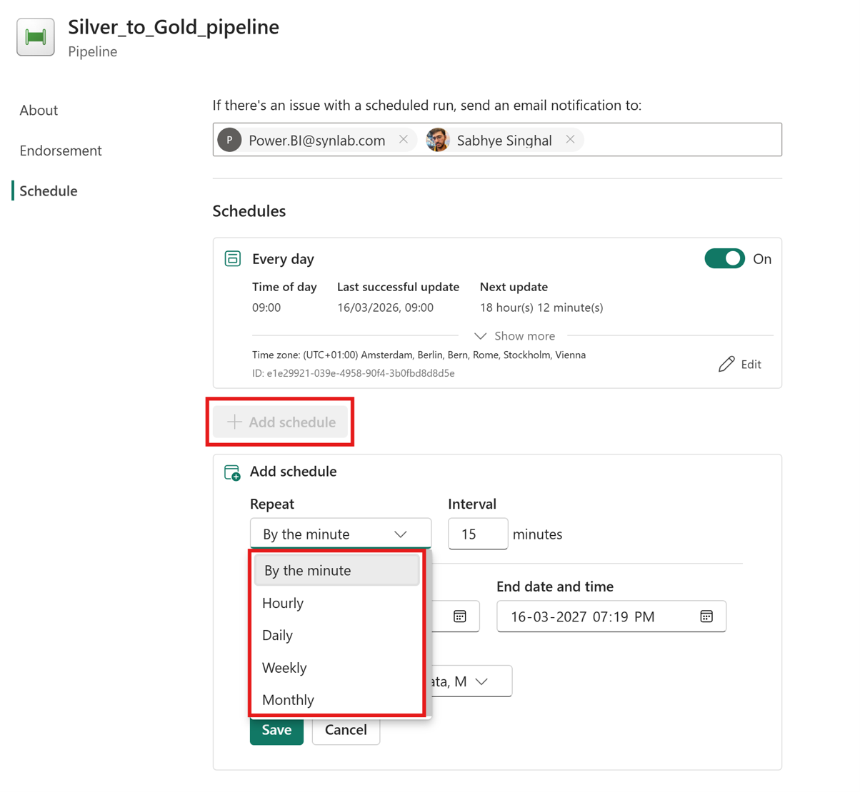
Click on add schedule. Based on your use case, you can schedule it by minute, hourly, daily, weekly or monthly. 

Pipeline schedule configuration showing frequency options from minute to monthly.

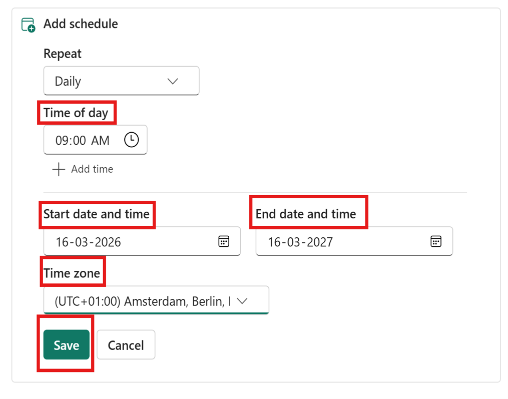
You can add the frequency. In our case, we need to run it on the daily basis. You can add attributes such as the time at which you want to schedule the pipelinestart date, end date and time zone. After this, click on save button.

Schedule settings set to run daily, with time, start date, end date and time zone fields.

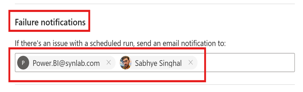
Also, you can add the email addresses at which the notification will be sent if the pipeline fails on a particular day.

Pipeline failure notification settings with email recipient fields.

OVERALL ARCHITECTURE

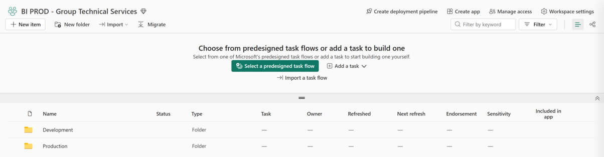
We have following 2 folders. Current architecture is under development folder.

BI PROD – Group Technical Services Fabric workspace showing the Development and Production folders.

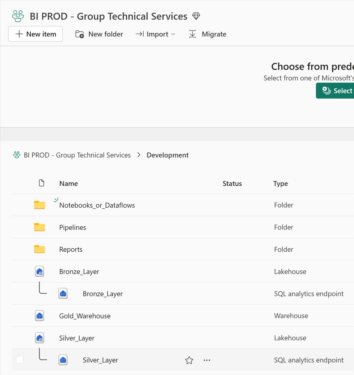
Under development folder, we will have following architecture. Our layers will be kept here. All the other items will be kept under respective folders. 

Development folder showing the Bronze and Silver lakehouses, Gold warehouse, and Notebooks, Pipelines and Reports subfolders.

Frequently Asked Questions (FAQ's)

Is it good to get data directly through dataflow Gen 2 or is it better to load the data first to Onelake using shortcuts and then reference that data to dataflow Gen 2?

Dataflow Gen2 pulls data directly from the source: 

Dataflow → Source system → Transform → OneLake 

Benefits: 

  • Simple end‑to‑end pipeline 
  • Less infrastructure to manage 
  • Good for operational/transactional sources that change frequently 
  • Good if you need to transform the data while loading 

Limitations: 

  • Repeatedly hitting the source system can cause: 
  • Load on transactional systems 
  • Throttling (e.g., Dataverse, SharePoint) 
  • Higher latency 
  • No centralized “source‑of‑truth” layer in OneLake 
  • Harder for other teams/tools to reuse the raw data 
  • You can’t reuse the same ingested dataset efficiently across multiple Dataflows 
Load to OneLake first (via shortcuts or ingestion), then let Dataflow Gen2 read from OneLake:

Source → OneLake shortcut/landing → Dataflow → curated data 

Benefits: 

  • Eliminates repeated source-system load 
  • Dataflow Gen2 reads local OneLake files, no external load. 
  • You get a reusable bronze layer 
  • Other teams/tools can use the same raw data 
  • Best for a lakehouse architecture 
  • Dataflow Gen2 fits nicely in Silver/Gold. 
  • Shortcuts make external data feel local 
  • You avoid copying data but still get: 
  • Local OneLake performance 
  • Delta format compatibility 
  • Ability to combine data from ADLS, S3, Dataverse, other workspaces 
  • Lower latency + higher stability 
  • Reading from OneLake is much faster than calling external APIs repeatedly.

Limitations: 

  • Requires an initial landing step (shortcut or separate ingestion) 
  • Slightly more architecture decisions 
  • Data freshness may depend on how often the source updates 

Hence second option will help in scalability, reusability, will be engine‑agnostic, useful for enterprise‑grade architecture. 

When to use medallion architecture?

You can use medallion architecture in following scenarios: 

  • When You Need a Reusable Raw Data Layer (Bronze) 
  • When Transformations Happen in Stages (Silver → Gold) 
  • When You Need Separation of Storage + Compute Layers 
  • When You Want Enterprise-Grade Architecture 


When not to use medallion architecture?

You cannot use medallion architecture in following scenarios: 

  • When Data Volumes Are Very Small or Simple 
  • When You Need RealTime or Near RealTime Streaming 
  • When Source System Direct Pull Is Simple and Does Not Cause Load 
  • When There Is No Need for Reusability Across Teams 
  • When You Don’t Need Warehousing or Star Schema Models 


Where shortcuts will work?

OneLake shortcuts only work with file-based object storage (S3/GCS/ADLS-style endpoints). 

Where shortcuts will won’t work?

SQL Server is not object storage, so it cannot be mapped as a shortcut. 

What are the alternatives if data is stored in SQL server?

Alternatives: 

  • Use Mirroring for SQL Server (Recommended) – It uses CDC and hence tables which fulfil CDC criteria will be copied. 
  • Use Dataflow Gen2 directly – Load time will increase 
  • Use Data Pipelines to load data to lakehouse 
What is mirroring?

Mirroring creates a real-time or near–real-time replica of your SQL Server tables into OneLake using CDC. 

Where can we use mirroring?

We should use mirroring: 

  • When the Source System Is SQL Server 
  • When You Need Near-Real-Time Sync 
  • When You Want to Avoid Full Loads 
Where can’t we use mirroring?

Tables excluded from mirroring: 

  • No primary key – CDC cannot track tables without PK 
  • Unsupported schema – FILESTREAM, in‑memory OLTP, sparse, computed columns 
  • Unsupported datatypes – CLR types, geography, geometry, sql_variant 
  • Temporal/history tables – Not supported by CDC-based mirroring 
  • Missing permissions – Fabric login lacks SELECT/ALTER ANY EXTERNAL MIRROR 
  • Already in replication – CDC conflict blocks mirroring 
  • System tables – Fabric mirrors user tables only 
What is data masking?

Data masking in Microsoft Fabric is a security feature that protects sensitive data by obscuring it for unauthorized or lowprivileged users, while still enabling analytics, reporting, and development work. 

Microsoft Fabric supports Dynamic Data Masking (DDM) natively in Fabric Data Warehouse and the SQL analytics endpoint. In our case, we are using Default mask (e.g., strings become XXXX, numeric become 0, dates become 1900-01-01). 

Who can view masked data?

Roles such as Admin, Member, or Contributor have CONTROL permission on the database by design and can view unmasked data by default. 

Who cannot view the masked data?

Users without the Administrator, Member, or Contributor rights on the workspace, and without elevated permissions on the Warehouse, will see masked data. 

What is the query to mask the data in a particular column?

– -Applying mask on a particular column – – 

ALTER TABLE dbo.pxo_validated_tickets 

ALTER COLUMN Id ADD MASKED WITH (FUNCTION = ‘default()’); 

GO 

– – Granting/Revoking permissions for a desired user on masked data column – – 

GRANT UNMASK ON dbo.pxo_validated_tickets TO sabhye.singhal@synlab.com; 

REVOKE UNMASK ON dbo.pxo_validated_tickets TO sabhye.singhal@synlab.com; 

– – Revoke permissions on a specific group – – 

ALTER ROLE <YourRoleName> REVOKE UNMASK;

What is row-level security?

Row-Level Security (RLS) in Microsoft Fabric allows you to restrict access to specific rows in a table based on who the user is or what role/group they belong to. This ensures each user sees only the data they’re permitted to see, even when everyone queries the same table. 

According to Microsoft Learn, RLS applies to both the Fabric Warehouse and the SQL analytics endpoint. 

RLS enables precise control by filtering rows at query time: 

  • Workers only see rows for their department 
  • Customers only see their organization’s data in a multitenant setup  

RLS is enforced inside the database tier, not in apps like Power BI, ensuring consistent security across all tools and reducing the risk of bypass.

In which scenarios RLS won't work?

Users with Admin, Member, or Contributor permissions at the workspace level inherently have highlevel control and can view unfiltered data. Also, if a table has no RLS policy, users see full unfiltered data.

What is the query to implement RLS on the data in a particular table?

– – Creating inline table-valued function – – 

Alter FUNCTION Security.country_securitypredicate(Country AS nvarchar(50)) 

    RETURNS TABLE 

WITH SCHEMABINDING 

AS 

    RETURN SELECT 1 AS country_securitypredicate_result 

WHERE @Country = ‘Germany’ AND USER_NAME() = ‘sabhye.singhal@synlab.com’; 

GO 


– – Using the function to create a Security Policy – – 

CREATE SECURITY POLICY filter_based_on_country 

ADD FILTER PREDICATE Security.country_securitypredicate(NOM_AGENCE) 

ON dbo.pxo_validated_tickets; 

GO 


– – Revoking the security policy – – 

Drop security policy filter_based_on_country